Learnable Soft Shrinkage Thresholds
In this work, we want to extend the soft-thresholding wavelet ideas initially introduced by Donoho and Johnstone in Ideal Spatial Adaptation by Wavelet Shrinkage, and later developed on by Chang, Yu and Vetterli in Adaptive Wavelet Thresholding for Image Denoising and Compression.
In particular, given a noisy image and its clean version as a target, is it possible to learn via backpropagation the soft shrinkage thresholds? How much better are they than by using the estimated thresholds from Chang et. al?
Note that this is a toy problem - I will be using the clean image as a target and use the MSE to backpropagate values to the thresholds. In general denoising problems we of course do not have access to the clean image. Perhaps we can estimate noise as a next step, but we will leave this for future work.
Background
Soft thresholding is a very popular and effective technique for denoising/compressing images. The basic technique involves:
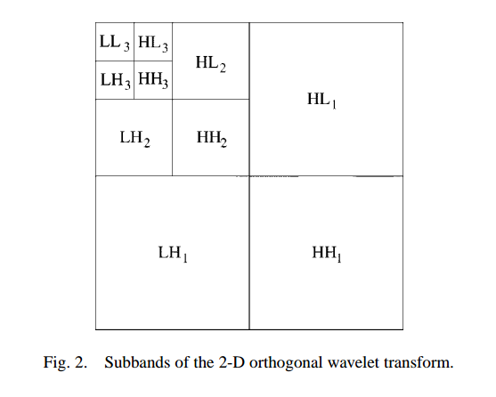
Taking a wavelet transform of the input - this has the advantage that the wavelet coefficients for most subbands of natural images are quite sparse.
Calculate a threshold \(T\) that will convert the noisy image \(Y=X+\epsilon\) to a denoised estimate \(\hat{X}\). Do this by minimizing the Bayes Risk
\[r(T) = E[(\hat{X}(T) - X)^2]\]
given some priors put on \(p(\epsilon)\) (a common one being that \(\epsilon \sim N(0, \sigma^2)\) - Use these thresholds on the wavelet bandpass coefficients (everything except from the LL output)
Reconstruct \(\hat{X}\) from the newly shrunk coefficients.
[1]:
# Import some plotting libraries
%matplotlib inline
%config InlineBackend.figure_format = 'svg'
import matplotlib as mpl
mpl.rcParams['savefig.dpi'] = 100
mpl.rcParams['figure.dpi'] = 100
import matplotlib.pyplot as plt
import matplotlib.gridspec as gridspec
from matplotlib.ticker import FormatStrFormatter
from PIL import Image
import plotters # Can be obtained from https://github.com/fbcotter/plotters

# Import our numeric libraries
import numpy as np
import torch
import torch.nn as nn

# import our wavelet libraries. pytorch_wavelets can be obtained from
# https://github.com/fbcotter/pytorch_wavelets
import pywt
from pytorch_wavelets import DTCWTForward, DTCWTInverse, DWTForward, DWTInverse

# Set the wavelet to be the Haar or Daubechies-1 wavelet
WAVE = 'db1'
[2]:
# Load in our image and create a noisy version
im = np.array(Image.open('trinity.jpg')).astype('float')
np.random.seed(100)
im_noise = im + 20 * np.random.randn(*im.shape)


fig, ax = plt.subplots(1,2, figsize=(8,4),
                       gridspec_kw=dict(left=0.01, right=0.99, top=0.99, bottom=0.01, hspace=0.01),
                       subplot_kw=dict(xticks=[], yticks=[]))
ax[0].imshow(plotters.normalize(im))
ax[1].imshow(plotters.normalize(im_noise))
ax[0].set_title('Original Image');
ax[1].set_title('Noisy Image');

[3]:
# Define our signal to noise ratio function
def mse(x, y):
    return np.mean((x-y)**2)

def snr(x, y):
    ϵ = y - x
    Ex = np.mean(ϵ)
    Ex2 = np.mean(ϵ**2)
    std = np.sqrt(Ex2 - Ex**2)
    σ = np.std(x)

    snr = 20*np.log10(σ/std)
    return snr

print('SNR on our noisy image is: {:.2f}dB'.format(snr(im, im_noise)))
SNR on our noisy image is: 12.67dB
Use Chang’s Threshold to Denoise
From equation 12 in Adaptive Wavelet Thresholding for Image Denoising and Compression, the wavelet soft thresholds that minimise the Bayes risk for the assumption that noise is gaussian are:
Where the \(B\) subscript indicates that this is a function of subband, \(\sigma_x\) is the variance of the noiseless wavelet coefficients, and \(\sigma\) is the variance of the noise.
Note that we can estimate \(\sigma\) robustly by calculating the median absolute deviation of the high-high wavelet coefficients at the finest level.
Then
[4]:
def bayes_thresh(im, J=3):
    """ Calculates the soft shrink thresholds for the 3 subbands of a J
    level transform. the input image can have more than one channel. The
    resulting array has shape T[J, 3, C], where:

    the zeroth dimension iterates over the J scales,
    the first dimension iterates over the bands LH, HL and HH, and
    the final dimension iterates over the C channels."""
    C = im.shape[-1]
    coeffs = pywt.wavedec2(im, WAVE, axes=(0, 1), level=J)
    bandpasses = coeffs[1:]

    # The indices of the different subbands
    lh_idx, hl_idx, hh_idx = 0, 1, 2

    # Estimate the noise variance using the median of the high-high wavelet coefficient
    # at the finest level. Repeat for each input channel.
    σ = np.zeros((C))
    for c in range(C):
        σ[c] = np.median(np.abs(bandpasses[J-1][hh_idx][:, :, c].ravel())) / .6745
    σ = σ.reshape(1, 1, C)

    # Estimate the variance of the noisy signal for each subband, scale and channel
    σy2 = np.zeros((J, 3, C))
    for j in range(J):
        for b in (lh_idx, hl_idx, hh_idx):
            for c in range(C):
                σy2[j, b, c] = np.mean(bandpasses[j][b][:, :, c]**2)

    # Calculate σ_x = sqrt(σ_y^2 - σ^2) for each subband, scale and channel
    σx = np.sqrt(np.maximum(σy2 - σ**2, 0.0001))

    # Calculate T
    T = (σ**2) / σx

    return T


def shrink(x: np.ndarray, t: float):
    """ Given a wavelet coefficient and a threshold, shrink """
    if t == 0:
        return x
    m = np.abs(x)
    denom = m + (m < t).astype('float')
    gain = np.maximum(m - t, 0)/denom
    return x * gain


def shrink_coeffs(coeffs: np.ndarray, T: np.ndarray):
    """ Shrink the wavelet coefficients with the thresholds T.

    coeffs should be the output of pywt.wavedec (list of numpy arrays)
    T should be an array of shape (J, 3, C) for color images.
    """
    assert T.shape[0] == len(coeffs) - 1
    J = len(coeffs) - 1
    assert T.shape[1] == len(coeffs[1])
    assert T.shape[2] == len(coeffs[1][0][0,0])
    C = T.shape[2]

    coeffs_new = [None,] * (J + 1)
    coeffs_new[0] = np.copy(coeffs[0])
    for j in range(J):
        coeffs_new[1+j] = [np.zeros_like(coeffs[1+j][0]),
                           np.zeros_like(coeffs[1+j][1]),
                           np.zeros_like(coeffs[1+j][2])]
        for b, band in enumerate(['LH', 'HL', 'HH']):
            for c in range(C):
                coeffs_new[1+j][b][:,:,c] = shrink(coeffs[1+j][b][:,:,c], T[j,b,c])

    return coeffs_new
Use the above to denoise the image
[5]:
T = bayes_thresh(im_noise)
coeffs = pywt.wavedec2(im_noise, WAVE, axes=(0,1), level=3)
x_hat = pywt.waverec2(shrink_coeffs(coeffs, T), WAVE, axes=(0,1))

# Plot the result
fig = plt.figure(figsize=(8,6))
gs = gridspec.GridSpec(2, 4, hspace=0.1, wspace=0.1, top=0.95, bottom=0.05)
ax1 = plt.subplot(gs[0,1:3], xticks=[], yticks=[], title='Input Image')
ax2 = plt.subplot(gs[1,:2], xticks=[], yticks=[],
                  title='Noisy Image\nMSE={:.2f}, SNR={:.2f}dB'.format(mse(im, im_noise), snr(im, im_noise)))
ax3 = plt.subplot(gs[1,2:], xticks=[], yticks=[],
                  title='Denoised Image\nMSE={:.2f}, SNR={:.2f}dB'.format(mse(im, x_hat), snr(im, x_hat)))
ax1.imshow(plotters.normalize(im))
ax2.imshow(plotters.normalize(im_noise))
ax3.imshow(plotters.normalize(x_hat));

Analysis and tests
How many elements are set to 0 across each of the subbands? Let us plot the distributions of the wavelet coefficients for three scales before and after shrinkage. For plotting purposes, we do not show the number of zeros in the shrunk coefficients as this will greatly outweigh all other values.
[6]:
#cA3, (cH3, cV3, cD3), (cH2, cV2, cD2), (cH1, cV1, cD1) = coeffs
J = 3
coeffs_unchanged = pywt.wavedec2(im_noise, WAVE, axes=(0,1), level=J)
shrunk_coeffs = shrink_coeffs(coeffs_unchanged, T)

def plot_hists(c1, c2, ax, ttl):
    bins = np.linspace(-2*c1.std(),2*c1.std(),50)
    ax[0].hist(c1.ravel(), bins=bins, color='r')
    ax[0].set_title(ttl)
    ylim = ax[0].get_ylim()

    keep_coeffs = np.abs(c2)>0
    ax[1].hist(c2[keep_coeffs].ravel(), bins=bins)
    ax[1].set_ylim(ylim)
    return keep_coeffs.sum()/keep_coeffs.size

for j in range(J):
    fig, ax = plt.subplots(3,2, figsize=(8,6), gridspec_kw={'hspace': .4})
    fig.suptitle('Scale {}'.format(J-j))
    for b, band in enumerate(['LH', 'HL', 'HH']):
        keep_percent = plot_hists(coeffs_unchanged[1+j][b][...,0],
                                  shrunk_coeffs[1+j][b][...,0], ax[b],
                                  ttl='{}, thresh= {:.1f}'.format(band, T[j,b,0]))
        ax[b,1].set_title('{:.1f}% coeffs are zero'.format(100*(1-keep_percent)))


We notice that the shrinking has a much larger impact on the finer coefficients. This is where it is easy to gain improvements in SNR as very little signal is here and a lot of noise.
Test commutativity
Because the inverse wavelet transform is linear, \(F(a+b) = F(a) + F(b)\).
MSE is obviously not linear though, so
The nice thing about orthogonal wavelets is that \(\sum_{i,j}F(a)F(b) = 0\), this means that \(L(a+b) = L(a) + L(b) + C\). Then, we can independently minimize each subband’s threshold.
Test linearity with subband coefficients
Annoyingly, we can only use haar for the moment. If we us another orthogonal wavelet, the subands are a bigger shape, and the above orthogonal property only holds when you set the right wavelet coefficients to nonzero.
[7]:
coeffs1 = pywt.wavedec2(im_noise, WAVE, axes=(0,1), level=J)
coeffs_zero = pywt.wavedec2(np.zeros_like(im_noise), WAVE, axes=(0,1), level=J)
# Set level 1 LH to be nonzero
coeffs_zero[1][0][:] = coeffs1[1][0]
ya = pywt.waverec2(coeffs_zero, WAVE, axes=(0,1))
# Set level 1 HL to also be nonzero
coeffs_zero[1][1][:] = coeffs1[1][1]
yab = pywt.waverec2(coeffs_zero, WAVE, axes=(0,1))
# Set level 1 LH to be nonzero
coeffs_zero[1][0][:] = np.zeros_like(coeffs1[1][0])
yb = pywt.waverec2(coeffs_zero, WAVE, axes=(0,1))
np.testing.assert_array_almost_equal(ya+yb, yab, decimal=5)
Test linearity with shrunk subband coefficients
[8]:
coeffs1 = pywt.wavedec2(im_noise, WAVE, axes=(0,1), level=J)
coeffs_zero = pywt.wavedec2(np.zeros_like(im_noise), WAVE, axes=(0,1), level=J)

# Set level 1 LH to be nonzero
coeffs_zero[1][0][:,:,0] = shrink(coeffs1[1][0][:,:,0], T[0,0,0])
ya = pywt.waverec2(coeffs_zero, WAVE, axes=(0,1))

# Set level 1 HL to also be nonzero
coeffs_zero[1][1][:,:,0] = shrink(coeffs1[1][1][:,:,0], T[0,1,0])
yab = pywt.waverec2(coeffs_zero, WAVE, axes=(0,1))

# Set level 1 LH to be nonzero
coeffs_zero[1][0][:,:,0] = np.zeros_like(coeffs1[1][0][:,:,0])
yb = pywt.waverec2(coeffs_zero, WAVE, axes=(0,1))
np.testing.assert_array_almost_equal(ya+yb, yab, decimal=5)
Test Orthogonality
Above I have stated that \(\sum_{i,j}F(a)F(b) = 0\). Let us test this
[9]:
coeffs_zero = pywt.wavedec2(np.zeros_like(im_noise), WAVE, axes=(0,1), level=J)
coeffs_zero[0][:] = np.random.randn(*coeffs_zero[0].shape)
ya = pywt.waverec2(coeffs_zero, WAVE, axes=(0,1))

coeffs_zero = pywt.wavedec2(np.zeros_like(im_noise), WAVE, axes=(0,1), level=J)
coeffs_zero[1][1][:] = np.random.randn(*coeffs_zero[1][0].shape)
yb = pywt.waverec2(coeffs_zero, WAVE, axes=(0,1))

coeffs_zero = pywt.wavedec2(np.zeros_like(im_noise), WAVE, axes=(0,1), level=J)
coeffs_zero[1][2][:] = np.random.randn(*coeffs_zero[1][0].shape)
yc = pywt.waverec2(coeffs_zero, WAVE, axes=(0,1))

coeffs_zero = pywt.wavedec2(np.zeros_like(im_noise), WAVE, axes=(0,1), level=J)
coeffs_zero[2][0][:] = np.random.randn(*coeffs_zero[2][0].shape)
yd = pywt.waverec2(coeffs_zero, WAVE, axes=(0,1))

coeffs_zero = pywt.wavedec2(np.zeros_like(im_noise), WAVE, axes=(0,1), level=J)
coeffs_zero[3][2][:] = np.random.randn(*coeffs_zero[3][2].shape)
ye = pywt.waverec2(coeffs_zero, WAVE, axes=(0,1))


np.testing.assert_array_almost_equal(np.sum(ya*yb), np.zeros_like(ya))
np.testing.assert_array_almost_equal(np.sum(ya*yc), np.zeros_like(ya))
np.testing.assert_array_almost_equal(np.sum(ya*yd), np.zeros_like(ya))
np.testing.assert_array_almost_equal(np.sum(ya*ye), np.zeros_like(ya))
np.testing.assert_array_almost_equal(np.sum(yb*yc), np.zeros_like(ya))
np.testing.assert_array_almost_equal(np.sum(yb*yd), np.zeros_like(ya))
np.testing.assert_array_almost_equal(np.sum(yb*ye), np.zeros_like(ya))
np.testing.assert_array_almost_equal(np.sum(yc*yd), np.zeros_like(ya))
np.testing.assert_array_almost_equal(np.sum(yc*ye), np.zeros_like(ya))
np.testing.assert_array_almost_equal(np.sum(yd*ye), np.zeros_like(ya))
Test Loss equations
[10]:
def mse_loss(x, x_hat=im):
    return np.mean((x-x_hat)**2)

# Calculate the mean removed image
coeffs = pywt.wavedec2(im_noise, WAVE, axes=(0,1), level=J)
coeffs_zero = pywt.wavedec2(np.zeros_like(im_noise), WAVE, axes=(0,1), level=J)
coeffs_zero[0] = np.copy(coeffs[0])
μ = pywt.waverec2(coeffs_zero, WAVE, axes=(0,1))
im2 = im - μ

# let F(a) be passing through level 1 LH
coeffs_zero = pywt.wavedec2(np.zeros_like(im_noise), WAVE, axes=(0,1), level=J)
coeffs_zero[1][0][:,:,0] = shrink(coeffs[1][0][:,:,0], T[0,0,0])
Fa = pywt.waverec2(coeffs_zero, WAVE, axes=(0,1))
La = mse_loss(Fa, im2)

# let F(b) be passing through level 1 HL
coeffs_zero = pywt.wavedec2(np.zeros_like(im_noise), WAVE, axes=(0,1), level=J)
coeffs_zero[1][1][:,:,0] = shrink(coeffs[1][1][:,:,0], T[0,1,0])
Fb = pywt.waverec2(coeffs_zero, WAVE, axes=(0,1))
Lb = mse_loss(Fb, im2)

coeffs_zero = pywt.wavedec2(np.zeros_like(im_noise), WAVE, axes=(0,1), level=J)
coeffs_zero[1][0][:,:,0] = shrink(coeffs[1][0][:,:,0], T[0,0,0])
coeffs_zero[1][1][:,:,0] = shrink(coeffs[1][1][:,:,0], T[0,1,0])
Fab = pywt.waverec2(coeffs_zero, WAVE, axes=(0,1))
Lab = mse_loss(Fab, im2)

np.testing.assert_almost_equal(Lab, La + Lb - np.mean((im2)**2))
To expand on the loss equations, consider \(L(a,b, \ldots , z)\). By simple induction, we can say
Where \(F(\mu)\) is the inverse wavelet transform of the non-zero mean coefficients (in our example, this is simply just the LL coefficients).
[11]:
coeffs = pywt.wavedec2(im_noise, WAVE, axes=(0,1), level=J)
coeffs_zero = pywt.wavedec2(np.zeros_like(im_noise), WAVE, axes=(0,1), level=J)

coeffs_zero[0] = coeffs[0]
Fμ = pywt.waverec2(coeffs_zero, WAVE, axes=(0,1))

coeffs_zero[1][0][:,:,0] = shrink(np.copy(coeffs[1][0][:,:,0]), T[0,0,0])
Faμ = pywt.waverec2(coeffs_zero, WAVE, axes=(0,1))
Laμ = mse_loss(Faμ)

coeffs_zero[1][1][:,:,0] = shrink(np.copy(coeffs[1][1][:,:,0]), T[0,1,0])
Fabμ = pywt.waverec2(coeffs_zero, WAVE, axes=(0,1))
Labμ = mse_loss(Fabμ)

coeffs_zero[1][0][:,:,0] = np.zeros_like(coeffs[1][0][:,:,0])
Fbμ = pywt.waverec2(coeffs_zero, WAVE, axes=(0,1))
Lbμ = mse_loss(Fbμ)

np.testing.assert_almost_equal(Labμ, Laμ + Lbμ - np.mean((im-Fμ)**2))
Plot MSE as a function of Threshold for each subband
This nice separability of the loss means we can minimize \(L(a)\) wrt \(T_a\), then do the same for \(L(b)\), and so on. This should give us a global minimum.
[12]:
# Iterate over all the subbands, setting all other thresholds to zero and find the
# MSE of the reconstructed images for a range of thresholds.
N = 20
J = 3
C = 3
mses = np.zeros((J,3,C,N))
T_mse = np.zeros((J,3,C))
Ts = np.zeros((J,3,C,N))
for j in range(J):
    for b, band in enumerate(['LH', 'HL', 'HH']):
        for c in range(C):
            coeffs = pywt.wavedec2(im_noise, WAVE, axes=(0,1), level=J)
            k = np.copy(coeffs[1+j][b][:, :, c])

            # Calculate 20 points from 0 to double the bayes estimated thresh
            Ts[j,b,c,:] = np.linspace(0, 3*min(T[j,b,c], .4*np.abs(k).max()), N)

            # Calculate the mse at the bayes estimate thresh
            coeffs[1+j][b][:,:,c] = shrink(np.copy(k), T[j,b,c])
            x_hat = pywt.waverec2(coeffs, WAVE, axes=(0,1))
            T_mse[j,b,c] = np.mean((x_hat - im)**2)

            # Calculate the mse at each of the N points
            for i,t in enumerate(Ts[j,b,c]):
                coeffs[1+j][b][:,:,c] = shrink(np.copy(k), t)
                x_hat = pywt.waverec2(coeffs, WAVE, axes=(0,1))
                mses[j,b,c,i] = np.mean((x_hat - im)**2)
Now that we have calculated the MSEs for a range of thresholds for each subband, plot the results
[13]:
colors = 'RGB'
c = colors.find('G')
T = bayes_thresh(im_noise)

fig, axes = plt.subplots(3, 3, sharey='row', figsize=(10, 10),
                         gridspec_kw=dict(left=0.1, right=0.96, top=0.96, bottom=0.1))
for j in range(J):
    for b, band in enumerate(['LH', 'HL', 'HH']):
        ax = axes[j, b]
        if b == 0:
            # Set the yticks for the first column
            ax.yaxis.set_major_formatter(FormatStrFormatter('%.2f'))
            ax0 = ax
            ax.set_ylabel('MSE', fontsize=16)
        else:
            plt.setp(ax.get_yticklabels(), visible=False)
            #ax.set_yticks(ax0.get_yticks())

        ax.plot(Ts[j,b,c], mses[j,b,c], label='MSE for subband soft threshold')

        if j == 0 and b == 1:
            ax.axhline(y=T_mse[j,b,c], ls='--',c='r',
                       label='MSE at bayes calculated thresh')
            ax.legend()
        else:
            ax.axhline(y=T_mse[j,b,c], ls='--',c='r')
        if j == J-1 and b == 1:
            ax.set_xlabel('Denoising Threshold t', labelpad=10, fontsize=16)

        ax.axvline(x=T[j,b,c], ls='--',c='r')
        ax.set_title('Scale {} {}'.format(J-j, band))
        #ax.set_xlim(0, max(Ts[j,b,c,-1], T[j,b,c]*1.1))

In the above plots, we set all the thresholds to 0 except the subband we are looking at. Note that all of the plots start at the noisy image’s MSE - 399.5. Then we independently increase the threshold for each subband and note the resulting MSE. Note that the largest gains are for the scale 1 (fine) coefficients.
The other interesting thing to note is that the bayes calculated threshold is very near the true minimum for almost all the subbands!
Convexity Test
Test the above assertion, that minimizing each threshold independently results in minimizing the overall MSE. First, search over the above plots for
[14]:
# Calculate T*
mse_min = np.argmin(mses, axis=-1)
T_star = np.zeros_like(T)
for j in range(J):
    for b in range(3):
        for c in range(C):
            T_star[j,b,c] = Ts[j,b,c, mse_min[j,b,c]]

# Calculate the MSE with T* vs with the bayes estimated thresholds
coeffs = pywt.wavedec2(im_noise, WAVE, axes=(0,1), level=J)
x_hat_min = pywt.waverec2(shrink_coeffs(coeffs, T_star), WAVE, axes=(0,1))
x_hat_bayes = pywt.waverec2(shrink_coeffs(coeffs, T), WAVE, axes=(0,1))
print('MSE using Bayes Shrink threshold is {:.2f}'.format(np.sum((im-x_hat_bayes)**2/im.size)))
print('MSE using optimal thresholds is {:.2f}'.format(np.sum((im-x_hat_min)**2/im.size)))
MSE using Bayes Shrink threshold is 85.43
MSE using optimal thresholds is 82.94
We haven’t really proven it’s the global minimum, but we have proven that it is at least better than using the bayes shrink thresholds.
Find threshold by gradients
Finite Differences
The above curve for \(L(T)\) looks quite smooth, so it seems plausible that the gradients are smooth. Let us test these via finite differences
[15]:
fig, ax = plt.subplots(1)

sample_j = 0
sample_band = 0
sample_channel = 1

ax.yaxis.set_major_formatter(FormatStrFormatter('%.2f'))
ax.plot(Ts[sample_j, sample_band, sample_channel], mses[sample_j, sample_band, sample_channel])
ax.set_title('LH subband for scale 3')
ax.set_xlabel('T')
ax.set_ylabel('L(T) - MSE')
plt.tight_layout()

[16]:
def F(t):
    coeffs = pywt.wavedec2(im_noise, WAVE, axes=(0,1), level=J)
    coeffs[1 + sample_j][sample_band][:, :, sample_channel] = \
        shrink(coeffs[1 + sample_j][sample_band][:, :, sample_channel], t)
    x_hat = pywt.waverec2(coeffs, WAVE, axes=(0,1))
    return x_hat

def L(t):
    return np.mean((im - F(t))**2)

def dLdt(T, dt=.1):
    return (L(T+dt) - L(T-dt))/(2*dt)

print('Gradient at T=5 is {:.4f}'.format(dLdt(5)))
print('Gradient at T=20 is {:.4f}'.format(dLdt(20)))
Gradient at T=5 is -0.0592
Gradient at T=20 is 0.0342
This matches up with the plotted curve
Manual backpropagation
Analytically what are the gradients?
by modifying \(T\)?
It is trivial to calculate \(\frac{dL}{d\hat{X}}\).
Calculating \(\frac{d\hat{X}}{dw}\) is not too difficult - simply need to take the forward wavelet transform with time reversed synthesis filters as the analysis filters. As we used orthogonal wavelets, this is already the case.
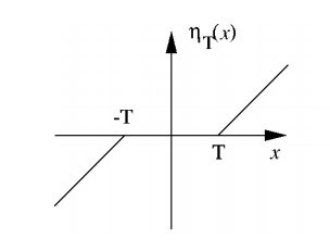
Calculating \(\frac{dw}{dT}\) is also trivial - I have done this already. To remind us, if:
then
and
[17]:
plt.figure()
t = 1.6
x = np.linspace(-5,5,100)
w = shrink(x, t)
dwdt = -np.sign(w)
plt.plot(x, w, label='w')
plt.plot(x, dwdt, label='dw/dt')
plt.legend(frameon=True)
plt.axhline(y=0, color='k', linewidth=.5)
plt.axvline(x=0, color='k', linewidth=.5)
plt.grid(ls='dashed')

[18]:
def dLdX_hat(x_hat, im):
    return 2*(x_hat-im)/x_hat.size

def dX_hatdw(x_hat):
    coeffs = pywt.wavedec2(x_hat, WAVE, axes=(0,1), level=J)
    return coeffs[1][0][:,:,1]

def dwdT(w, T):
    coeffs = pywt.wavedec2(im_noise, WAVE, axes=(0,1), level=J)
    g = shrink(coeffs[1][0][:,:,1], T)
    g = -np.sign(g)
    return np.sum(g*w)

def np_backprop(T):
    return dwdT(dX_hatdw(dLdX_hat(F(T), im2)), T)

print('Gradient at T=5 is {:.4f}'.format(np_backprop(5)))
print('Gradient at T=20 is {:.4f}'.format(np_backprop(20)))
Gradient at T=5 is -0.0592
Gradient at T=20 is 0.0342
autograd (using pytorch)
Pytorch does have its own soft thresh function, but it only gives gradients w.r.t the input.
To work around this, we have to define our own autograd function for the soft threshold which gives gradients w.r.t. the input and the thresholds:
[19]:
from torch.autograd import Function
class SoftShrink_fn(Function):
    @staticmethod
    def forward(ctx, x, t):
        y = nn.functional.softshrink(x, t.item())
        ctx.save_for_backward(torch.sign(y))
        return y

    @staticmethod
    def backward(ctx, dy):
        din, = ctx.saved_tensors
        dx, dt = None, None
        if ctx.needs_input_grad[0]:
            dx = dy * din * din
        if ctx.needs_input_grad[1]:
            dt = -torch.sum(dy * din)
        return dx, dt

class SoftShrink(nn.Module):
    def __init__(self, t_init):
        super().__init__()
        self.t = nn.Parameter(torch.tensor(t_init))

    def forward(self, x):
        """ Applies Soft Thresholding to x """
        return SoftShrink_fn.apply(x, self.t)

from torch.autograd import gradcheck
x = torch.randn(10,10, requires_grad=True, dtype=torch.double)
t = torch.tensor(1., requires_grad=True, dtype=torch.double)
gradcheck(SoftShrink_fn.apply, (x,t))
[19]:
True
Use this to calculate the gradient at \(T=5\) and \(T=20\) as we did for the finite differences above
The DWT from pytorch_wavelets behaves slightly differently to pywt.wavedec2. The latter returns its decomposition as a list of coeffs, where coeffs[0] is the lowpass, coeffs[1] is the coarsest or Jth scale bandpass, and coeffs[-1] is the finest or first scale banpass coefficients.
DWTForward returns a tuple of (yl, y_bandpass) where y_bandpass[0] is the finest scale coefficients and y_bandpass[-1] is the coarsest.
[20]:
dwt = DWTForward(J=3, wave=WAVE)
iwt = DWTInverse(wave=WAVE)
X = torch.tensor(im.astype('float32').transpose((2,0,1))[None,:])
Y = torch.tensor(im_noise.astype('float32').transpose((2,0,1))[None,:],
                 requires_grad=True)

shrinker = SoftShrink(0.0)

def F_torch(T):
    # Shrink the LH of the first scale
    yl, yh = dwt(Y)
    shrinker.t.data = torch.tensor(T)
    c = shrinker(yh[J-1-sample_j][0, sample_channel, sample_band])
    yh[J-1-sample_j][0, sample_channel, sample_band] = c
    return iwt((yl, yh))

def L_torch(T):
    return torch.mean((X - F_torch(T))**2)

y = L_torch(5.0)
y.backward(retain_graph=True)
print('Gradient at T=5 is {:.4f}'.format(shrinker.t.grad.item()))
shrinker.t.grad.zero_()
y = L_torch(20.0)
y.backward(retain_graph=True)
print('Gradient at T=20 is {:.4f}'.format(shrinker.t.grad.item()))
Gradient at T=5 is -0.0592
Gradient at T=20 is 0.0342
Good! this agrees with the finite differences approximation to the gradient. Now that we have a function to calculate gradients, let us minimize!
Optimize
We will need to slightly modify the above softshrink function to work with channels of input:
[21]:
class SoftShrink_ch_fn(Function):
    @staticmethod
    def forward(ctx, x, t, C):
        y = torch.zeros_like(x)
        for c in range(C):
            for i in range(3):
                y[:,c,i] = nn.functional.softshrink(x[:,c,i], t.data[c,i])
        ctx.save_for_backward(torch.sign(y))
        return y

    @staticmethod
    def backward(ctx, dy):
        din, = ctx.saved_tensors
        dx, dt = None, None
        if ctx.needs_input_grad[0]:
            dx = dy * din * din
        if ctx.needs_input_grad[1]:
            dt = -torch.sum(dy * din, dim=(0,3,4))
        return dx, dt, None

class SoftShrink_ch(nn.Module):
    def __init__(self, C, t_init, t_grad=True):
        super().__init__()
        assert t_init.shape[-1] == 3
        assert t_init.shape[0] == C
        self.t = nn.Parameter(torch.tensor(t_init).float())
        self.constrain = nn.ReLU()
        self.C = C

    @property
    def thresh(self):
        return self.constrain(self.t)

    def forward(self, x):
        """ Applies Soft Thresholding to x """
        if x.shape == torch.Size([0]):
            return x
        else:
            assert x.shape[1] == self.C
            return SoftShrink_ch_fn.apply(x, self.thresh, self.C)

x = torch.randn(1,3,3,4,4, dtype=torch.double, requires_grad=True)
t = torch.rand(3,3, dtype=torch.double, requires_grad=True)
y = SoftShrink_ch_fn.apply(x, t, 3)
gradcheck(SoftShrink_ch_fn.apply, (x,t,3))
[21]:
True
Now that we have this, create the ‘net’ that shrinks coefficients:
[22]:
class MyThresh(nn.Module):
    def __init__(self, t_init=None):
        super().__init__()
        if t_init is None:
            t_init = np.random.rand(3,3,3)
        self.dwt = DWTForward(J=3, wave=WAVE)
        self.iwt = DWTInverse(wave=WAVE)
        self.shrinkers = nn.ModuleList([
            SoftShrink_ch(C=3, t_init=t_init[0]),
            SoftShrink_ch(C=3, t_init=t_init[1]),
            SoftShrink_ch(C=3, t_init=t_init[2])
        ])

    def forward(self, x):
        coeffs = self.dwt(x)
        coeffs[1][0] = self.shrinkers[0](coeffs[1][0])
        coeffs[1][1] = self.shrinkers[1](coeffs[1][1])
        coeffs[1][2] = self.shrinkers[2](coeffs[1][2])
        y = self.iwt(coeffs)
        return y
[23]:
def get_lr(optim):
    lrs = []
    for p in optim.param_groups:
        lrs.append(p['lr'])
    if len(lrs) == 1:
        return lrs[0]
    else:
        return lrs

def minimize(T_init=None):
    DeNoise = MyThresh(T_init)
    optimizer = torch.optim.Adam(DeNoise.parameters(), lr=2e-0)
    #scheduler = torch.optim.lr_scheduler.MultiStepLR(
    #    optimizer, milestones=[120, 180, 220], gamma=0.5)
    criterion = torch.nn.MSELoss(reduction='elementwise_mean')
    for step in range(250):
        #scheduler.step()
        optimizer.zero_grad()
        Z = DeNoise(Y)
        mse = torch.mean((X - Z)**2)
        loss = criterion(Z,X)
        if torch.isnan(mse):
            raise ValueError('Nan encountered in training')
        if step % 10 == 0:
            print('Step [{:02d}]:\tlr: {:.1e}\tmse: {:.2f}'.format(
                step, get_lr(optimizer), mse.item()))
        loss.backward()
        optimizer.step()
    return DeNoise
[24]:
Denoise = minimize()
/home/fergal/.pyenv/versions/3.6.6/lib/python3.6/site-packages/torch/nn/_reduction.py:13: UserWarning: reduction='elementwise_mean' is deprecated, please use reduction='mean' instead.
  warnings.warn("reduction='elementwise_mean' is deprecated, please use reduction='mean' instead.")
Step [00]:      lr: 2.0e+00     mse: 386.94
Step [10]:      lr: 2.0e+00     mse: 118.08
Step [20]:      lr: 2.0e+00     mse: 88.08
Step [30]:      lr: 2.0e+00     mse: 84.94
Step [40]:      lr: 2.0e+00     mse: 84.00
Step [50]:      lr: 2.0e+00     mse: 83.62
Step [60]:      lr: 2.0e+00     mse: 83.29
Step [70]:      lr: 2.0e+00     mse: 83.12
Step [80]:      lr: 2.0e+00     mse: 83.03
Step [90]:      lr: 2.0e+00     mse: 82.99
Step [100]:     lr: 2.0e+00     mse: 82.96
Step [110]:     lr: 2.0e+00     mse: 82.94
Step [120]:     lr: 2.0e+00     mse: 82.92
Step [130]:     lr: 2.0e+00     mse: 82.91
Step [140]:     lr: 2.0e+00     mse: 82.90
Step [150]:     lr: 2.0e+00     mse: 82.88
Step [160]:     lr: 2.0e+00     mse: 82.88
Step [170]:     lr: 2.0e+00     mse: 82.87
Step [180]:     lr: 2.0e+00     mse: 82.86
Step [190]:     lr: 2.0e+00     mse: 82.85
Step [200]:     lr: 2.0e+00     mse: 82.85
Step [210]:     lr: 2.0e+00     mse: 82.84
Step [220]:     lr: 2.0e+00     mse: 82.84
Step [230]:     lr: 2.0e+00     mse: 82.83
Step [240]:     lr: 2.0e+00     mse: 82.83
Plot the new thresholds compared to the bayes threshold ones:
[25]:
colors = 'RGB'
c = colors.find('R')
T = bayes_thresh(im_noise)

plt.figure(figsize=(10,10))
gs = gridspec.GridSpec(3,3)
gs.update(left=0.1, right=0.95, wspace=0.05, hspace=.2, top=0.95)
for j in range(J):
    for b, band in enumerate(['LH', 'HL', 'HH']):
        if b == 0:
            ax = plt.subplot(gs[j,b])
            ax.yaxis.set_major_formatter(FormatStrFormatter('%.2f'))
            ax0 = ax
        else:
            ax = plt.subplot(gs[j,b])
            plt.setp(ax.get_yticklabels(), visible=False)

        ax.plot(Ts[j,b,c], mses[j,b,c])
        if j == 0 and b == 1:
            ax.axvline(x=T[j,b,c], ls='--',c='r',
                       label='Bayes calculated thresh')
            ax.axvline(x=Denoise.shrinkers[2].t[c,1], ls='--', c='g',
                       label='Backprop calculated thresh')
            ax.legend(framealpha=1)
        else:
            ax.axvline(x=T[j,b,c], ls='--',c='r')
            ax.axvline(x=Denoise.shrinkers[J-1-j].t[c,b], ls='--', c='g')

        ax.set_title('Scale {} {}'.format(J-j, band))
        ax.set_xlim(0, max(Ts[j,b,c,-1], T[j,b,c]*1.1))

It works! We have learned the optimal thresholds via backpropagation. As mentioned at the beginning of this notebook however, this is still not ideal as we needed the noiseless image to calculate the MSE.